Practical Hints for Investment Analysis
Everybody likes Tips & Tricks! In this section, we will present some useful hints that will help you create smart investment analysis.
The topics:
More topics to come soon!
How to compare the profitability of projects with different economic life?
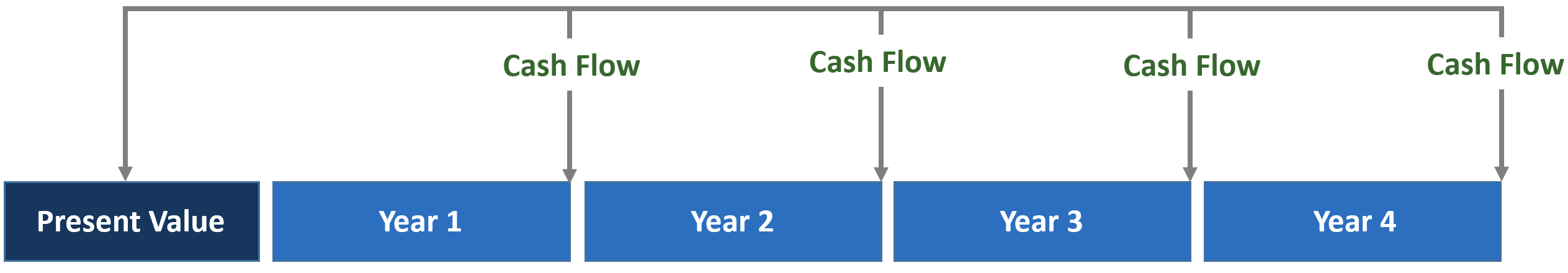
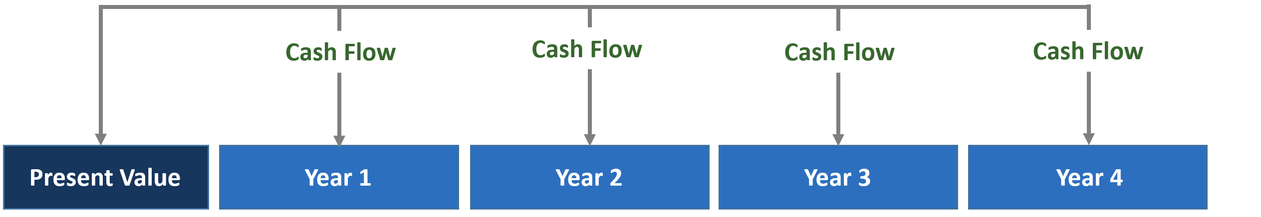
As the NPVs of two or more investments with different economic life are not directly comparable, a monthly annuity payment of NPV can be used as the basis for comparison. The decision-making rule: The higher the monthly annuity payment, the better the investment is.
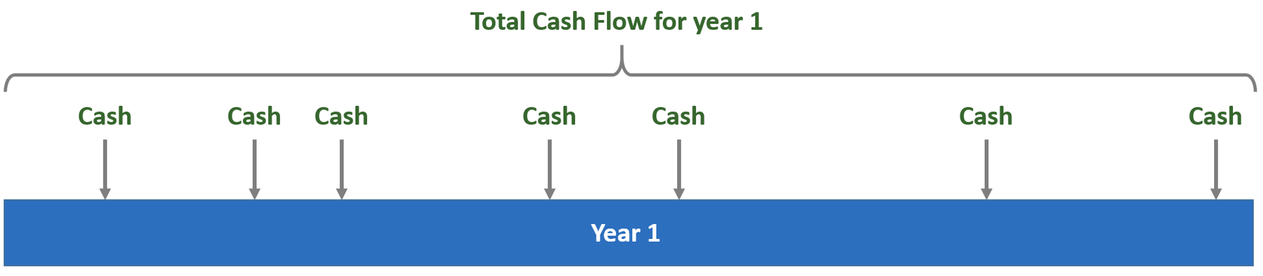
Annuity payments are a series of future constant payments based on a constant discounting rate so that the sum of their present value is equal to the project’s NPV.
For example:
What is the yearly annuity of this project, calculated against its NPV?
|
Present
moment
|
Year 1 |
Year 2 |
| Free Cash Flows |
-100 |
70 |
120 |
NPV = -100 + 70/((1+10%)^1) + 120/((1+10%)^2) = 63
Answer:
The yearly annuity for this project constituting of 2 payments in year 1 and year 2 is 36, as:
36/((1+10%)^1) + 36/((1+10%)^2) = 63 = NPV
Annuity payments corresponding to the Example Project:
|
Present
moment
|
Year 1 |
Year 2 |
|
Yearly Annuity
Payments
|
0 |
36 |
36 |
Exercise with us!
We need to compare two investment alternatives, one with the economic life of 3 years and the other – of 4 years. Let’s determine projects’ NPVs.
PROJECT 1:
Annual discount rate = 2,75%
|
Present
moment
|
Year 1 |
Year 2 |
Year 3 |
| FCF |
-10 000 |
10 000 |
9 000 |
12 000 |
NPV = 19 319
PROJECT 2:
Annual discount rate = 2,75%
|
Present
moment
|
Year 1 |
Year 2 |
Year 3 |
Year 4 |
| FCF |
-12 000 |
7000 |
8 000 |
8 000 |
14 000 |
NPV = 22 325
The Project 2 returns higher NPV, however, it also lasts 1 year longer in comparison to Project 1. With the Invest for Excel® software, it is easy to determine the monthly annuity and use it as the proper comparison indicator.
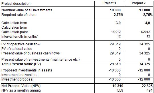
The calculation shows that despite lower NPV, the monthly annuity is higher of the Project 1!
Download the Invest for Excel® test version now and test it for proper comparisons of the projects with different life-cycles. You can use the above example as your exercise! If you have any questions, please contact us and we will be glad to help.
What is Sensitivity Analysis and how to use it?
Introduction
Sensitivity analysis is aimed at reducing the uncertainty in the evaluation of investment models.
Usually, sensitivity analyses are calculations for studying how alternative assumptions in the various variables affect profitability. The analysis can be used for studying when an investment becomes unprofitable or which assumptions make a difference between two profitable alternatives with regard to their profitability.
Sensitivity analyses give an idea how the profitability of an investment project is affected by changing certain basic assumptions or values (e.g. the acquisition cost increases by 10%, or variable costs decrease by 5%).
We will present here the most common ways of performing sensitivity analysis in investment models or business projects. We will not include in this article the probabilistic methods that require more insightful explanation.
Single-parameter sensitivity analysis
Single-parameter sensitivity analysis helps to reveal the impact how changes in a certain parameter affect the total model results.
In Invest for Excel software, the ready spreadsheet called Analysis is present in all calculation files. It displays the charts range that shows sensitivity of key variables (one variable at the time): Discount rate, total investments, income, variable costs, fixed costs, specific parameter of income variables can be additionally selected by the user.
The outcome results can also be selected by the reviewer – for example: NPV, IRR, MIRR, Payback, DCVA and more.
For example:
Picture 1:The sensitivity analysis chart inbuilt in every calculation file of Invest for Excel software.
- Sensitivity analysis - Spider diagram
It helps to determine which are the key drivers that shape the model outcome. The customized charts can be easily created by the user via opening a dialog window and selecting desired parameters for analysis. There will be automatically a new spreadsheet added with the customized sensitivity chart.
For example:
Picture 2: Spider diagram – impact of variables with up to 30% change on NPV
The chart above shows that a 15% drop in production output leads to negative NPV. The chart also shows that the NPV still would be positive although variable- or fixed costs would increase with 30%.
- Sensitivity analysis - Tornado diagram
The Tornado chart demonstrates the impact that a fixed change in each parameter has on the main model results. Both the input and output parameters can be selected by the user. For example, this diagram clearly depicts that Income variable has the greatest influence on determining project’s NPV.
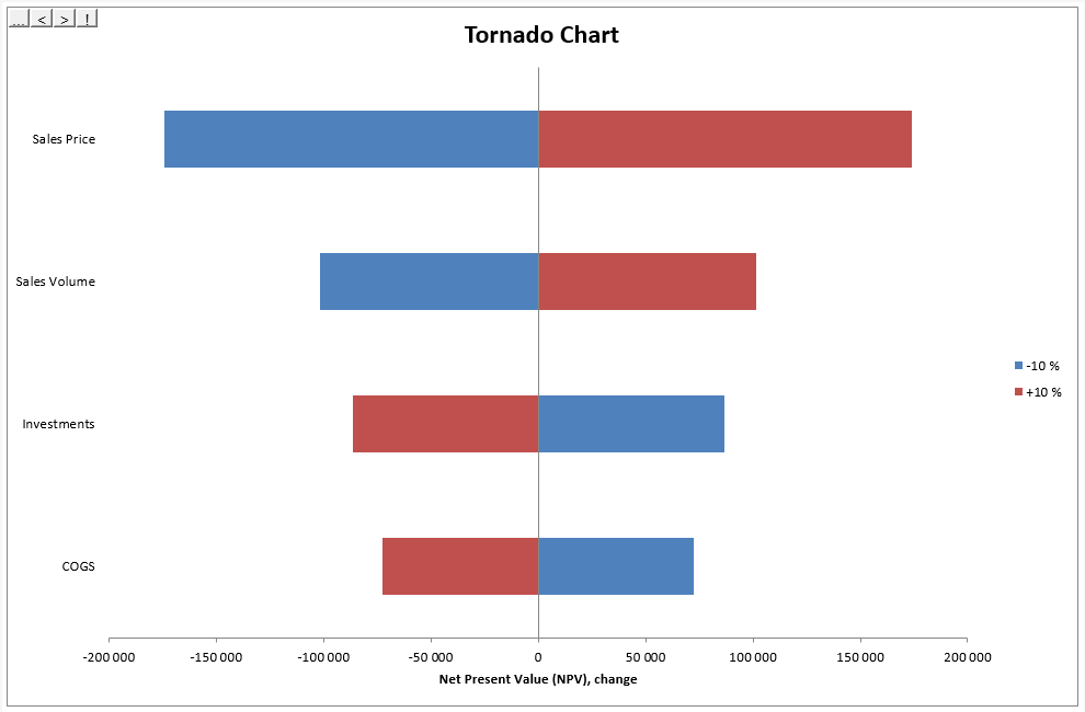
Picture 3: Tornado diagram – how the change of variables by 10% impacts the outcome: NPV
- Break-even function – important sensitivity feature
By running the Break-Even function, you can quickly calculate the break-even point of the investment on any input parameter - for example how much certain incomes can drop, or costs rise, while the NPV falls to zero level, meaning that if implemented with the given target interest rate, the investment would, theoretically, only just be feasible.
Example:
What is the minimum price (break-even), so that project stays profitable (NPV =0)?
Picture 4: Searching break-even value for Price parameter
The break-even value was found for Price parameter. It is important to notice that the parameter level for all periods over the time was found, not just for the first period:
Picture 5: Break-even value for Price parameter is found and relevant for all calculation periods.
Multiple-parameter sensitivity analysis
Such analysis allows for examining the relationship of two or more different parameters changing at the same time, at a given range that can vary individually per each parameter. It shows how each potential combination of the changed parameters affect the model’s results. The reviewer can determine this way the results of most optimistic scenario, the most pessimistic scenario and all the range of options between those extremes.
While using Invest for Excel® software, the user can utilise standard MS Excel environment with calculation files created in the software. The multiple-parameter sensitivity analysis is supported by Scenarios Manager function.
Example:
This analysis depicts how 2 parameters changing simultaneously (price and efficiency) affect profitability result: NPV and IRR.
Picture 6: Multiple-parameter sensitivity analysis table
Download the Invest for Excel® test version now and test it for multi-range of sensitivity analysis!
If you have any questions, please contact us and we will be glad to help: Phone: +358 19 54 10 100, E-mail: [email protected]
How to model financing of the project?
While taking decision on how to finance a project, there are many typical questions that need to be addressed:
- How much financing is needed?
- What type of loan will be the most appropriate (annuity, equal amortizations, bullet, customized repayment scheme)?
- What repayment period is feasible (and which one is certainly not)?
- How to model drawdown, repayment, financing costs of a loan and integrate it to the cash flow of the project?
- Is there an effect on tax?
- What is an effect on financial statements of adding financing (Cash flow, Balance Sheet etc.)?
With Invest for Excel® software, all these questions can be answered in minutes as the Enterprise edition includes a Financing module that helps to develop suitable financing scheme as well as integrate it with the investment calculation. The financing module includes such valuable features as:
- Based on input of several loan parameters, the whole financing plan is created “on click” with exact cash flows of withdrawals, fees, interest and debt change, incorporating capability for various currencies, floating rates, various types of loans, consolidation of loans and more.
- The Financing model can be exported to Investment Calculation “on click” and the Financial Statements of the Investment calculation are updated accordingly. For example Income Statement with the Financing Items, Balance Sheet with the Debt Change, Cash Flow Statement with all debt service. The tax effects of Financing items or capitalization of financing expenses can be also included – as standard options.
- The financing files of Invest for Excel® can be used as a loan register.
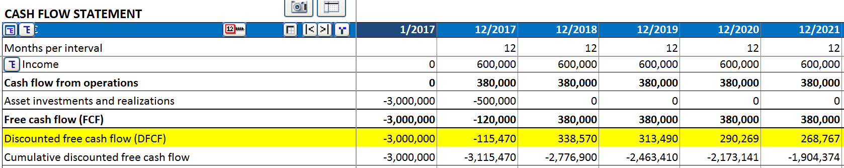
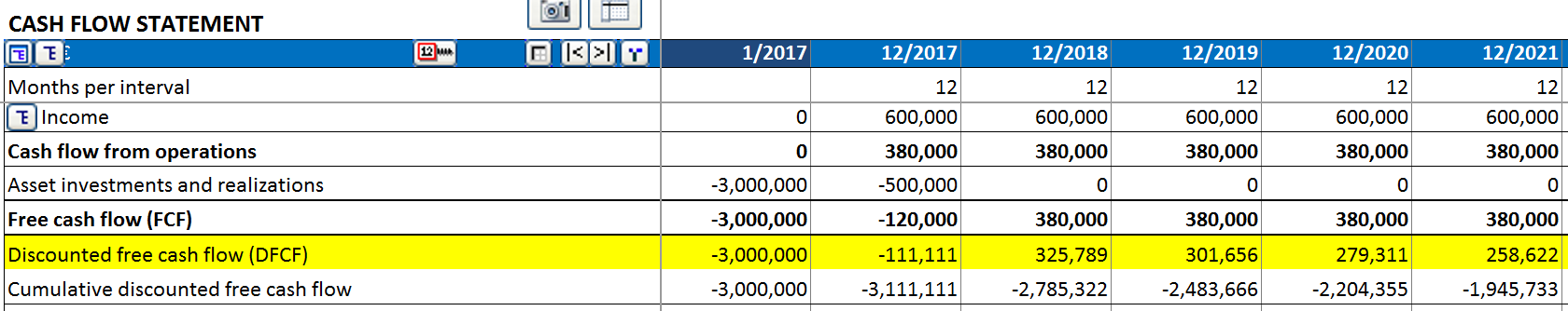
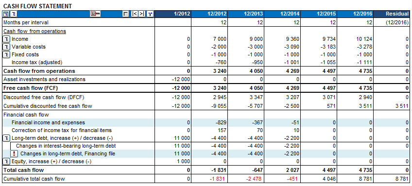
When planning financing, we should start by analyzing the Project Cash Flow (View: Cash flow Statement in the Investment File). Example:
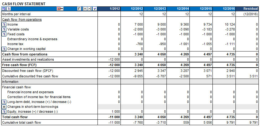
Picture 1. Cash flow statement of a project (Investment file)
The Cumulative total cash flow – the last line of the statement shows the need of debt financing of 11 000 for 1/2012. It is time to open Financing module and start analyzing financing alternatives.
From the Homescreen of Invest for Excel® program, select Financing and create a new File.
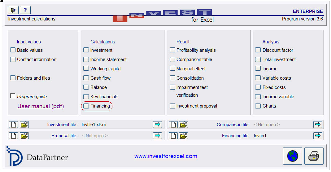
Picture 2. Homescreen of Invest for Excel® software with the available menu of functionalities.
The Financing file can be updated with the Project cash flow from the Investment file, just with one click.
The financing file has a convenient structure that allows the user to easily navigate and input all necessary parameters such as drawdown, interest, fees, time of repayment etc.
Below, there is an example how the parameters have been chosen for financing the project case study.
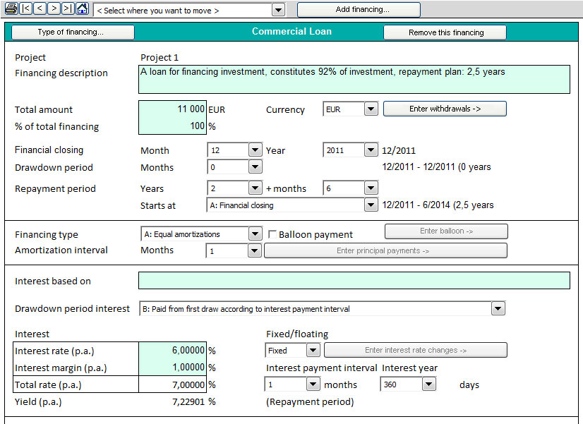
Picture 3. Parameters of the loan (Financing file)
Loan parameters:
- Interest rate: 6%
- Margin: 1%
- Type of loan: Equal amortizations
- Drawdown on financial closing: 12/2011
- Repayment: 2,5 year
After entering loan withdrawal, the fees, loan interest and loan principal repayments are calculated.
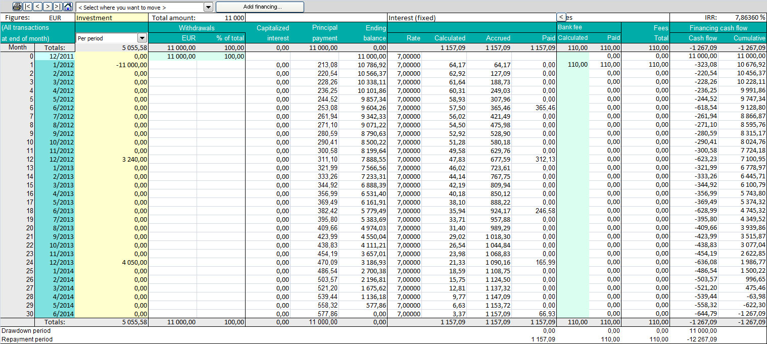
Picture 4. The detailed specification of the loan withdrawal, interest, fees, repayment and also project cash flows – view month by month (Financing file)
Several summary reports are generated, such as:
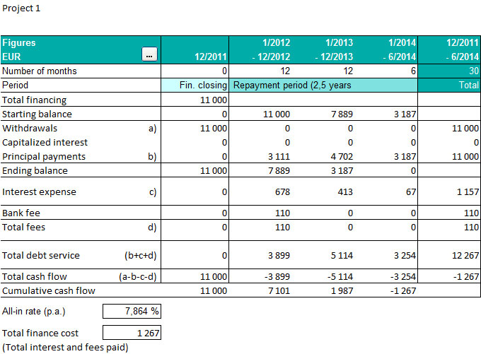
Picture 5. Summary view (Financing file)
When the financing cash-flows are determined, the next step is to combine them with the project cash flows and verify if the selected option is feasible. No need of copying or moving the columns or even linking the files. It is easy to update Investment calculation file with projected financing using the button with the red exclamation mark. Done!
Picture 6. Cash flow statement of the project, including financing – option 1 (Investment file)
The changes in debt and financing costs are highlighted with light-blue colour. As the cash flow statement depicts it, the choice of financing is unsatisfactory in that case. In the first years the project has negative cumulative cash flow, which may suggest that the desired repayment period of 2,5 years is too short.
Let’s extend the loan repayment to 4 years and find out if this type of financing is suitable.
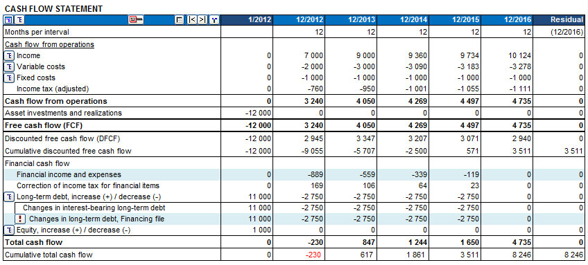
Picture 7. Cash flow statement of the project, including financing – option 2 (Investment file)
As a result, the cumulative total cash flow is still slightly negative. There can be several solutions: the type of repayment can be changed from equal amortizations to annuity, the repayment period extended or simply the amount of financing should be slightly increased, to be prepared for the upcoming interest. Below, the first option is selected and it shows that the change of a loan type to annuity, with 4 years repayment period is a good plan for financing this project. The Cumulative total cash flow is positive, which states that the financing is sufficient.
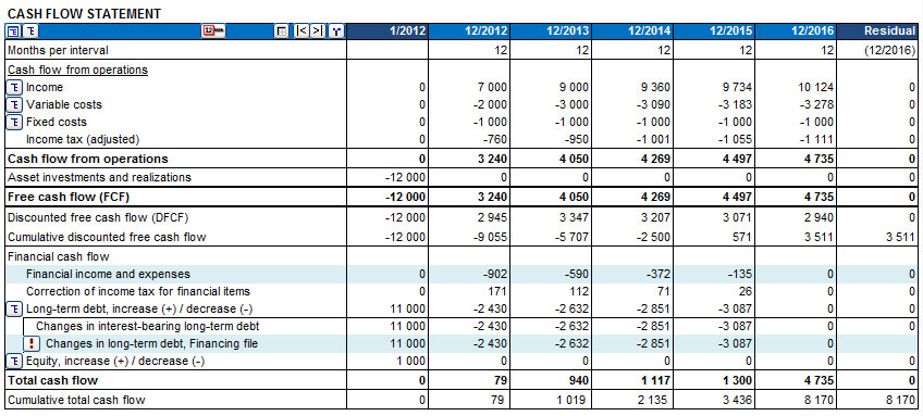
Picture 8. Cash flow statement of the project, including financing – option 3 (Investment file)
With financing cash flows integrated with the investment cash flows, it is possible to analyze the project’s profitability from the FCFE viewpoint and get the leverage effect on NPV to Equity. The risk vs. return of financing can be assessed.
The debt may be aggregated from several loans. You can add loans by pressing the "Add financing.." -button.
Financing Module is available in the Enterprise edition of Invest for Excel®.
If you have any questions, please contact us and we will be glad to help you: Phone:+358 19 54 10 100, E-mail: [email protected]
Two ways to deal with marginal effects of investments
Very often an investment is of the kind that it in some form improves current operations. It may save in costs for energy, raw materials, personnel or logistics. It may increase capacity or quality. Anyway the effect of the investment is marginal. How to calculate the effect it brings?
Way one
1) Typically a marginal investment calculation is done. Example: A production facility consumes a substantial amount of electricity. A 100 000 Euro additional investment in energy saving equipment would give a power saving of 30 000 Euros per year in 5 years. A simple calculation gives an IRR of 15,24% before taxes. Fair enough, but reality is seldom this simple.
Wouldn’t the power saving be depending on production volumes? Would the installation of this equipment cause a break in production? Would the additional investment affect other costs? How would it affect working capital and taxes?
Way two
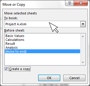
2) The alternative way is to deal with “the whole picture”. First, model your current operations. Then save the calculation file with a new name. Include the additional investment and all its effects carefully to this calculation file, so that the effects are depending on volumes etc. Then use the “Marginal effect” function in Invest for Excel® software to create a comparison calculation:
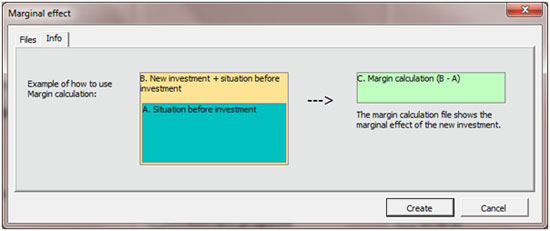
In the upper “A”-field, select the calculation file of current production, without additional investment. In the lower “B”-field, select the calculation file including additional investments.
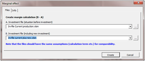
Open files can be selected with the drop down menu (arrow on the right). Saved files can be selected by pressing the button with three dots, on the right side:
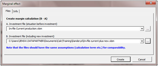
Note that the two files compared should have the same discount rate, calculation term and tax assumptions for comparability.
When you press Create –button a third calculation file will be created automatically. This will be the marginal investment calculation. This new calculation would then be the investment appraisal for the new investment, showing only the marginal changes. Basically the result should be exactly the same as the handmade marginal calculation, Example 1, in the beginning of this article. However, sometimes working with the “whole picture” gives a more exact result. It is because it brings more aspects for considerations and helps avoid simplifications. This functionality makes it easier to create marginal calculations in complex situations. This is the most common way to calculate investments in process industries and manufacturing.
Another advantage of this method is that you also can compare “current situation” with “current plus new investment” using Comparison table function in Invest for Excel® software.
If you have any questions, please contact us and we will be glad to help you: Phone:+358 19 54 10 100, E-mail: [email protected]
How to demonstrate extreme scenarios in Sensitivity analysis? You can include changes of several variables at the same time and create a chart
The sensitivity analysis charts typically display the change for only one variable at a time and the assumption is that the rest of variables stay unchanged. For example: what if investments increase +/- 10% and all other variables such as costs or incomes are without any changes.
Invest for Excel is helpful in demonstrating extreme effects in What-if Analysis, considering the impact of several variables altogether.
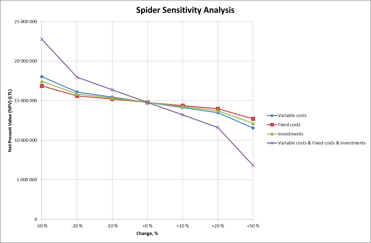
"Show line with all changes combined" option is available in the Spider analysis chart.
It is possible to combine the effects of sensitivity changes on up to 5 variables selected by the user. As a result, the line chart showing all the changes combined will be displayed in addition to the one-variable sensitivity line charts. In the below example, the line chart showing all the changes combined is of the violet colour and includes +/- changes of: Variable costs AND Fixed costs AND Investments altogether, providing the overview of the project profitability in extreme positive and negative scenarios.
Available in the software compilation 3.6018 and newer.
How to handle Residual Values in Invest for Excel®
Residual Value
An important question to consider when making investment calculations is the Residual Value. The Residual Value is how much a fixed asset is worth at the end of its useful life. The term Salvage Value is used in accounting. Salvage Value is the estimated value that an asset will realize upon its sale at the end of its useful life. The value is used in accounting to determine depreciation amounts or can be determined by a regulatory body such as the IRS. However the Asset Book Value at the end of the calculation period used when making financial projections typically differ from the market value. Thus you need to adjust the Residual Value in the Residual column of Invest for Excel®.
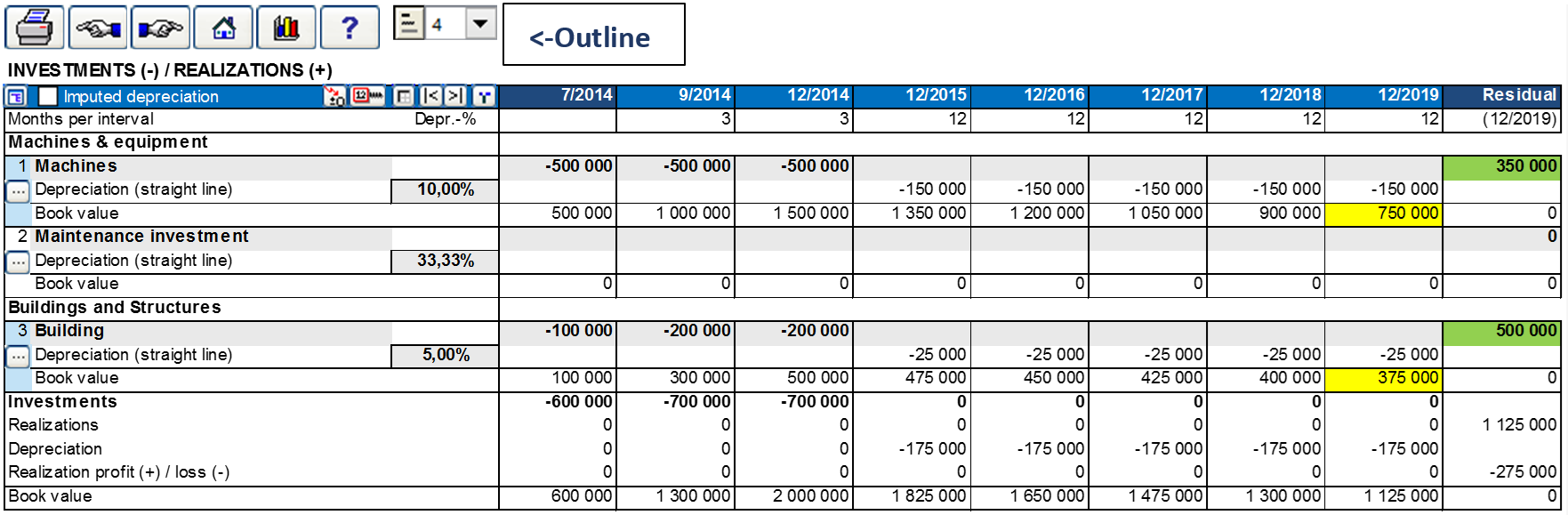
Picture 1, investments table in Invest for Excel. Hint: When changing Outline level from 3 to 4 the book values of each asset is shown. The yellow cells show the Asset Book Values at the end of the calculation period. Also the green cells show by default the Asset Book Values at the end of the period, but these values can (and should) be adjusted to market value. This is done simply by typing, replacing the formula in the green cells. Notice that changing the residual value will give Realization profit/ loss, which will be included in the Income Statement.
The size of the Residual Value is of course very much depending of the term of calculation. In theory you should make the calculation term the same as the Economic Life of the main investment object. The Economic Life being the expected period of time during which an asset is useful to the average owner. The Economic Life of an asset could be different than the actual physical life of the asset.
In reality the calculation term is often shorter than the Economic Life. This can be due to practical reasons, e.g. you have a better overview of 10 columns, than 40, or you do not want to make forecasts beyond 5 years, or the standard calculation period in your corporation’s investment appraisals is set to be 10 years. Any of the above reasons increases the need for assessing the real Residual Value. Remember that the Residual Value also can be negative, e.g. demolition-, environmental cleaning- or restoration costs.
Different types of assets behave differently, technological equipment might lose value quite fast, whereas a residential building could increase in value. Please remember the time value of money when you enter the residual value. Example: if you assume a 2% annual value growth for a building over 10 years, use this formula to calculate the residual value: -investment * (1+2%)^10.
No Residual Value
Because of caution, or because of company guidelines you might not include any residual values. In Invest for Excel you have 3 optional ways not to include residual.
- Enter “0” for residual value in Residual column. This results potentially in a Realization loss in Income Statement but has no cash effects.
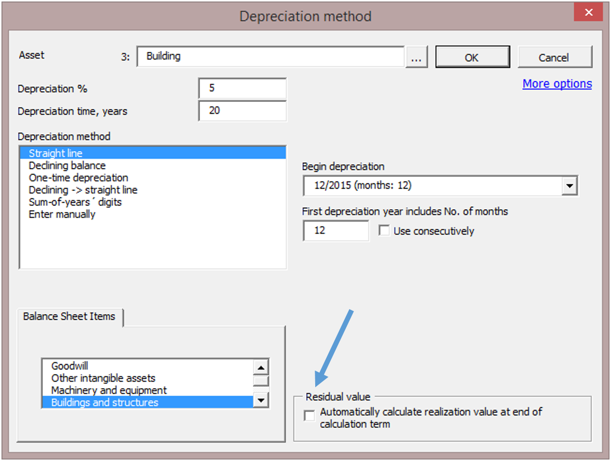
- Unselect the option “Automatically calculate realization value at the end of calculation term”, which you can find in the “Depreciation method” dialog box. When this option is deselected there will be no realization at the end, and thus no profit/loss. The asset simply stays in the Balance sheet. See Picture:
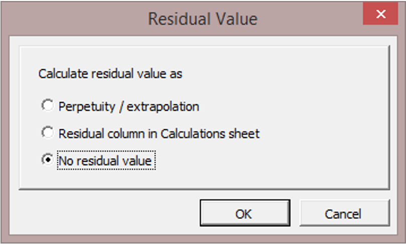
- Select “No residual value” option in the “Residual value” dialog box. This dialog box is available in the “Calculation term” dialog box accessed from “Basic Values” screen and in “Profitability analysis” screen on “Result” sheet. Note! This function is available only in the Enterprise version. When this option is selected there is no residual column at all in the calculation. See Picture:
Extrapolation
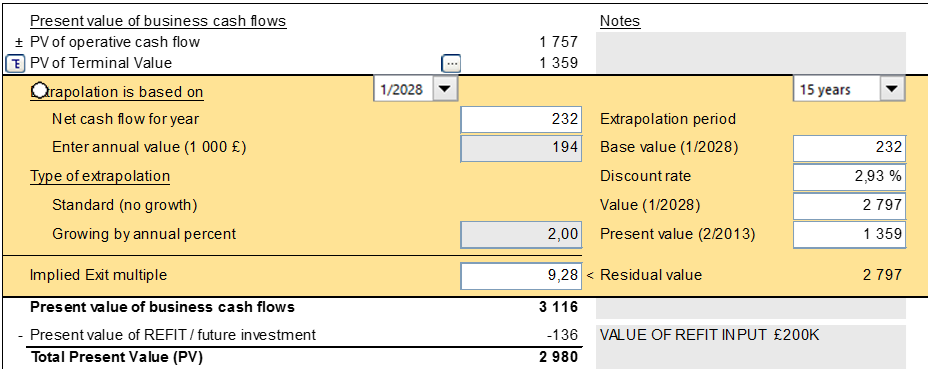
The Extrapolation function extends the cash flows beyond the original scope. Example: You are modelling an object with 40 year Economic Life with a stable income stream, e.g. a power grid. Instead of modelling 40 years, you could model the 10 first years and then extrapolate the next 30 years, assuming some steady development. This function is available only in the Enterprise edition of Invest for Excel. This is how you do it:
In the Residual Value dialog box, select Perpetuity / extrapolation:
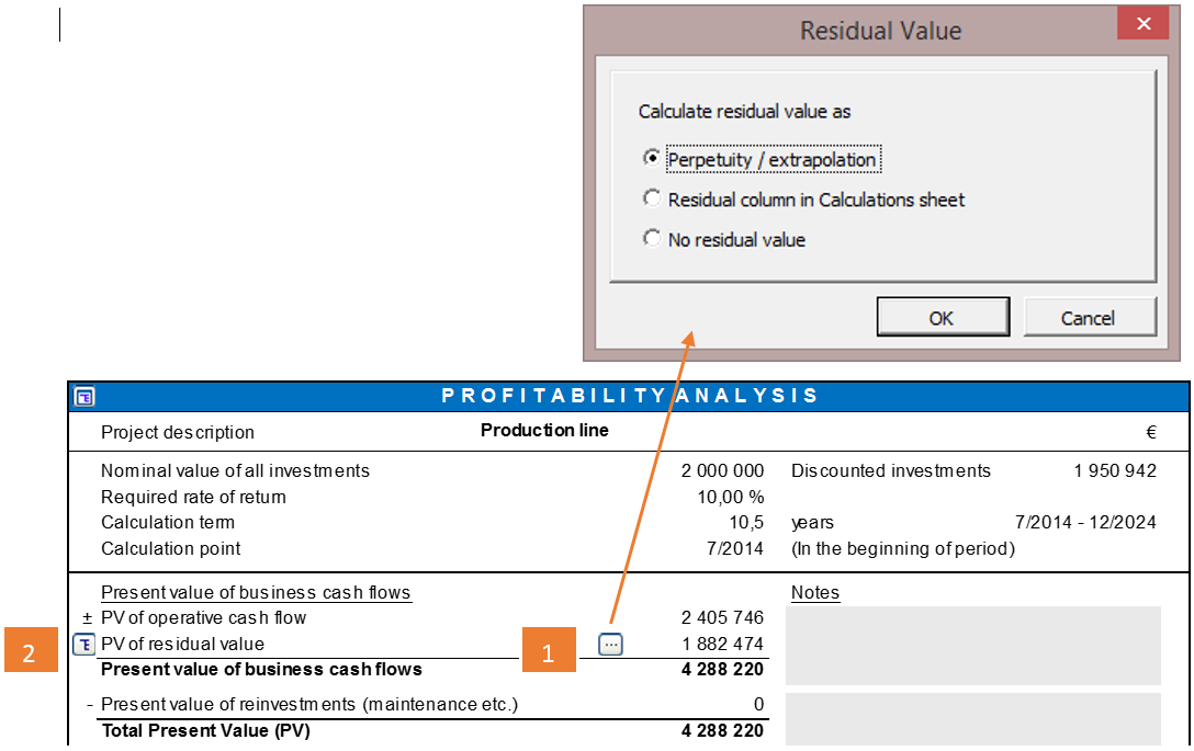
Then press 2nd button at left to open the settings for calculation of Continuing Value (PV of residual value). See picture:
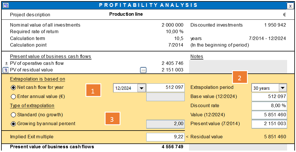
1) Select year or enter cash flow to base the extrapolation on
2) To the right change from Extrapolation period “Perpetual” to “30 years”
3) Choose between no growth or choose “Growing by percent”. The growth percent can also be negative.
Going Concern
Going Concern means assuming that a business entity will continue to operate in the foreseeable future without the need or intention on the part of management to liquidate the entity or to significantly curtail its operational activities. In other words, we assume that the business will continue indefinitely.
In Invest for Excel® we use the term Perpetuity. A perpetuity is a stream of cash payments that continues forever. The Perpetuity function is available only in the Enterprise edition of Invest for Excel®.
Perpetuity is used when valuating companies and business operations and very often for real estate valuations as well.
Example:
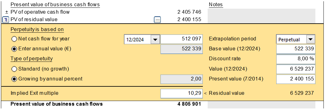
Hint: You may base the Perpetuity on an 11th year by choosing “Enter annual value”, then entering a formula that multiplies the 10th year’s Net cash flow with 1+growth% (see above).
Hint: The “Implied Exit multiple” tells you how many last year’s EBITDAs, the Value (12/2024) equals. E.g. Implied Exit multiple 10 tells us that the Residual Value equals 10 year’s EBITDA.
Hint: Some Microsoft Excel versions cause a problem, when the buttons lose their places. It could the look like this:
The fix is to run the “Arrange buttons” function found in the “Format” menu of Invest for Excel:
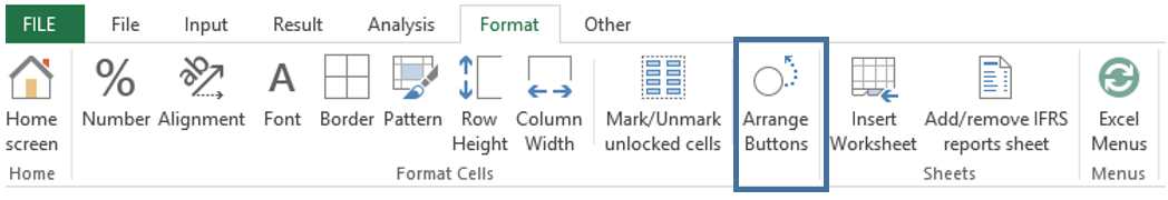
The Arrange buttons function puts the workbook’s all buttons back in place!